All controls

Every control on the Scanpath page, where it is and what it does — in the order you meet them on screen. Search this page (Ctrl+F, or Cmd+F on a Mac) for the thing you want to change, such as colors, legends or axes.

The page has two sets of controls:

• The trial control bar, above the plot, decides what you see: the dataset, the trial, and which trials are in the list.
• The plot controls, the column on the right, decide how it is drawn: each layer of the figure, its colors and sizes, and the figure as a whole.

The tabs under the plot then work with the trial on screen: annotate it, read its context, compare it, export it or share it. For how the parts fit together, see the Scanpath visualization guide.

For the corresponding Python keywords and CLI flags, use the figure options table.

Trial control bar

The bar above the plot: pick a dataset and a trial, step through the trials, and narrow, sort or label the list.

Control	What it does
Select dataset	The dataset the page shows.
+ → Create manually	Add a dataset by manual illustration: write a text and place its fixations by hand.
+ → Import files	Add a dataset from data tables: upload your own tables as a new dataset.
Select trial	The trial to show. Click it and type to narrow the list.
Trial slider	Scrub through the trials in the list.
◀ ▶	The previous or next trial.
⇅ → Sort trials by	Reorder the trial list by a statistic (such as reading time), a participant, text or condition field, or a column of a metadata table you attached.
⇅ → Descending	Reverse that order.
→ Text / Participant	Keep only these texts or participants.
→ a field of your data	Keep only trials with these values, or, for a number, in this range.
→ By participant / By trial / By text	The same, for the columns of an attached metadata table.
→ Favorites only	Keep only starred trials.
→ With any of these tags	Keep only trials with any of these tags.
→ Excluding tags	Hide trials with any of these tags, such as exclude.
→ Clear all filters	Reset every filter in the panel.
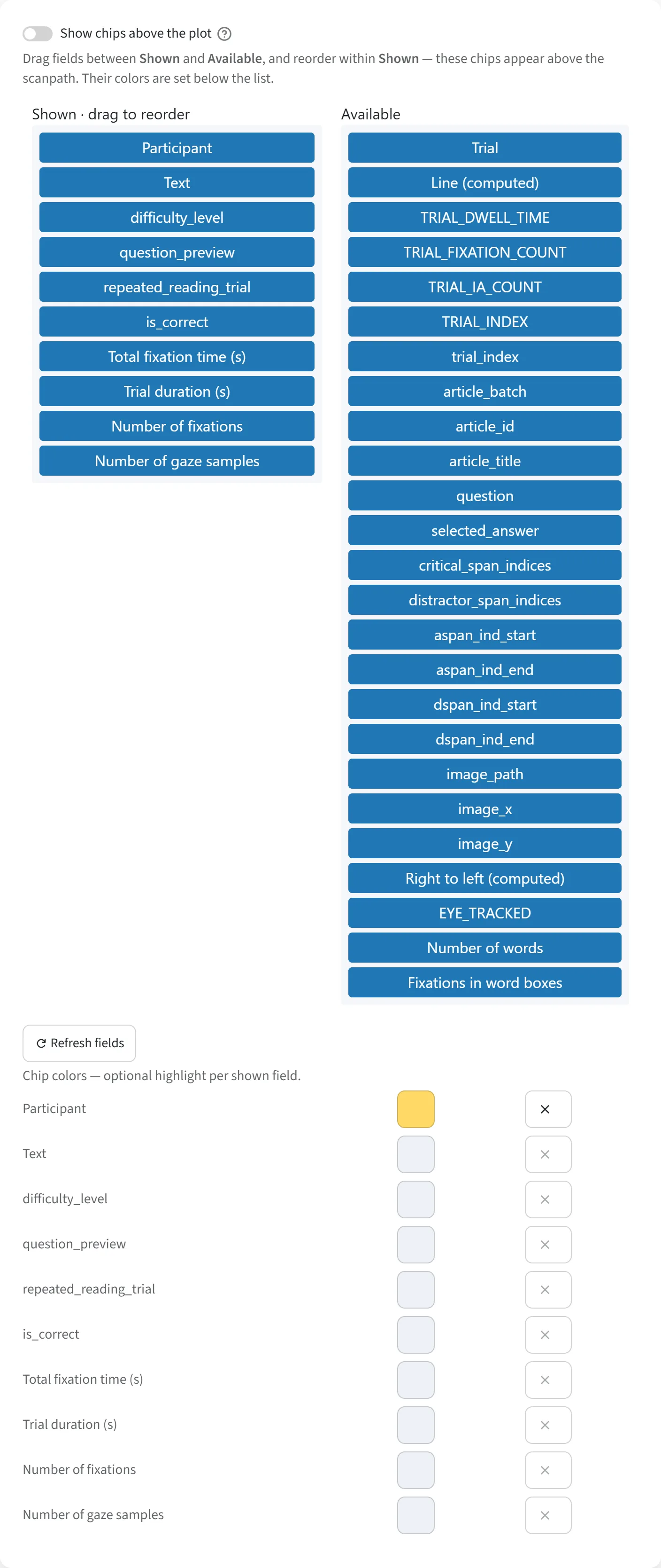
✏️ → Show chips above the plot	Show or hide the row of facts about the trial above the plot.
✏️ → field lists	Drag fields between Shown and Available to choose the chips. Available holds every field with one value per trial: participant, text and condition columns, the columns of any metadata table you attached, and statistics such as reading time and fixation count.
✏️ → field colors	Give a chip a highlight color; its ✕ puts it back to the default gray.
✏️ → Refresh fields	Look again for which fields are trial-level.
Screen and its ◀ ▶	On a trial recorded over several screens: the screen to show.

Plot controls

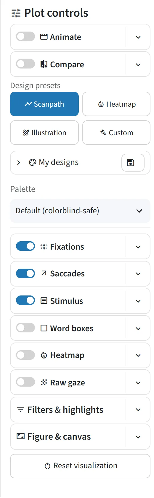
The column on the right of the plot. At the top, the modes and designs change the whole figure at once. Under them, each layer of the figure has a row of its own: the switch turns the layer on or off, and the ▾ beside it opens that layer's settings, described below one menu at a time. The last two rows, Filters & highlights and Figure & canvas, cover the figure as a whole. A greyed-out control says why when you hover over it.

Animate: play the reading as a video

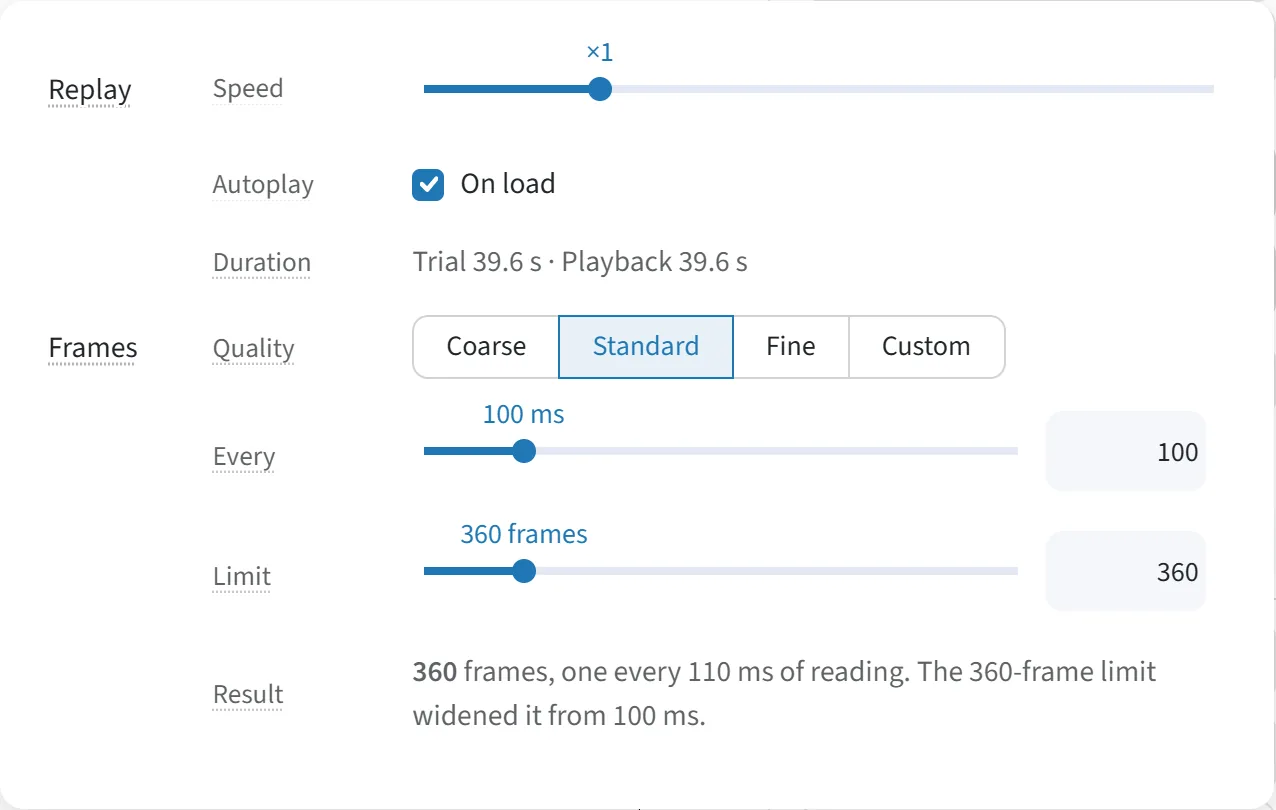
The Animate switch turns the figure into an animation, a video of the reading played back fixation by fixation, with play and pause buttons and a time slider under the plot. Its ▾ holds:

Control	What it does
Replay → Speed	How fast the video plays, from ×0.25 to ×8: ×1 is the reader's own pace, ×2 twice as fast, ×0.5 half as fast.
Replay → Autoplay → On load	Start playing the animation automatically as soon as the plot is shown; otherwise it starts only when you click play.
Replay → Duration	For information only: the trial's reading time, and how long the video runs at this speed.
Frames → Quality	How smooth the video is: more frames play more smoothly but take longer to build. Custom sets the two below by hand.
Frames → Every	Reading time between frames, in ms.
Frames → Limit	The most frames a video gets; a long trial gets wider frame steps to fit.
Frames → Result	For information only: how many frames this trial's video has, and how far apart they ended up.

Compare

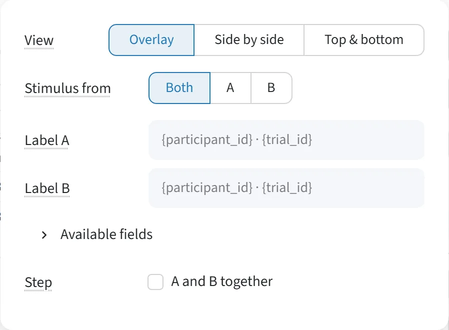
The Compare switch shows a second scanpath, B, beside or over this one (pick it in the trial control bar, above the plot); its ▾ holds:

Control	What it does
View	Overlay both scanpaths, or give each its own panel, Side by side or Top & bottom.
Stimulus from	In an overlay, whose word boxes and text are drawn: both, A's or B's.
Label A / Label B	Each scanpath's name in the legend, written with fields such as {participant_id}; empty uses the automatic one.
Available fields	The fields a label can use.
Step → A and B together	◀ ▶ move both scanpaths at once.

Design presets and palette

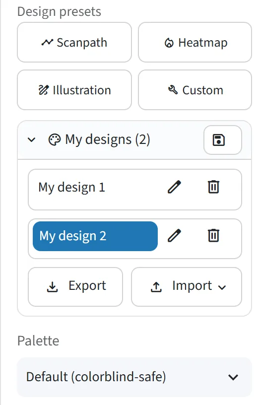
Restyle the whole figure in one click, with a ready-made design or one of your own saved designs:

Control	What it does
Scanpath / Heatmap / Illustration	Ready-made designs: a classic scanpath, a word-box heatmap, or a clean schematic.
Custom	Your most recent hand-made settings.
My designs	Your saved designs: click one to apply it; the pencil renames it and the bin deletes it.
My designs → save button	Save the settings on screen as a named design, to apply again later in one click.
My designs → Export / Import	Download your designs as a file, or load a file of designs: share a look with co-authors and partners, reproduce a figure exactly, or move your designs to another computer.
Palette	A color scheme for the whole figure, such as colorblind-safe or print.

Fixations

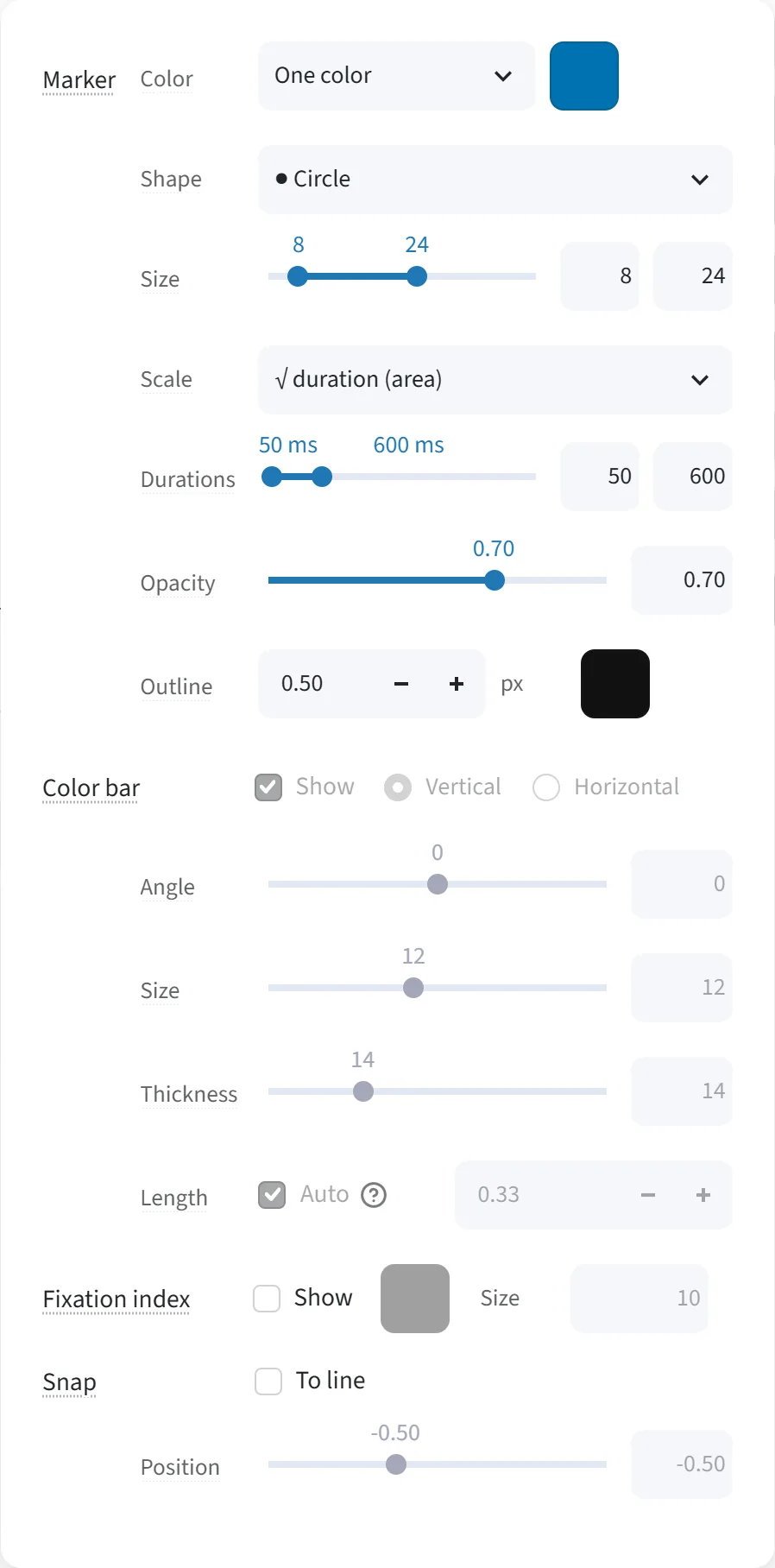
The Fixations switch draws the fixation markers; its ▾ holds:

Control	What it does
Marker → Color	What decides each marker's color. One color paints them all alike. Pick a number column of the fixations, such as duration or the fixation's order in the trial, and the markers follow a color scale: with the default blues, longer fixations show darker. Pick a category, such as the line of text or the next saccade's direction, and each value gets its own color, with a legend.
Marker → color box	Choose the fixation marker color.
Marker → Shape	Choose the fixation marker shape: circle, square, diamond, triangle, star…
Marker → Size	Set the marker size range: the smallest and largest marker diameter, in px.
Marker → Scale	Choose how duration sets marker size: square root, linear, log, or relative to the trial.
Marker → Durations	Choose the duration range: set the durations that get the smallest and the largest marker.
Marker → Opacity	Set the fixation marker opacity; lower it to see overlapping fixations.
Marker → Outline	Set the width and color of the ring round each marker.
Color bar → Show	Show the color scale's bar, when markers are colored by a number.
Color bar → orientation, Angle, Size, Thickness, Length	Set the bar's direction, tick-label angle and size, and its thickness and length.
Fixation index → Show	Number each fixation in reading order.
Fixation index → color, Size	Choose the numbers' color and size.
Snap → To line	Move each fixation onto its line of text — a schematic, labelled Illustration.
Snap → Position	Choose where on its line a snapped fixation sits.

Saccades

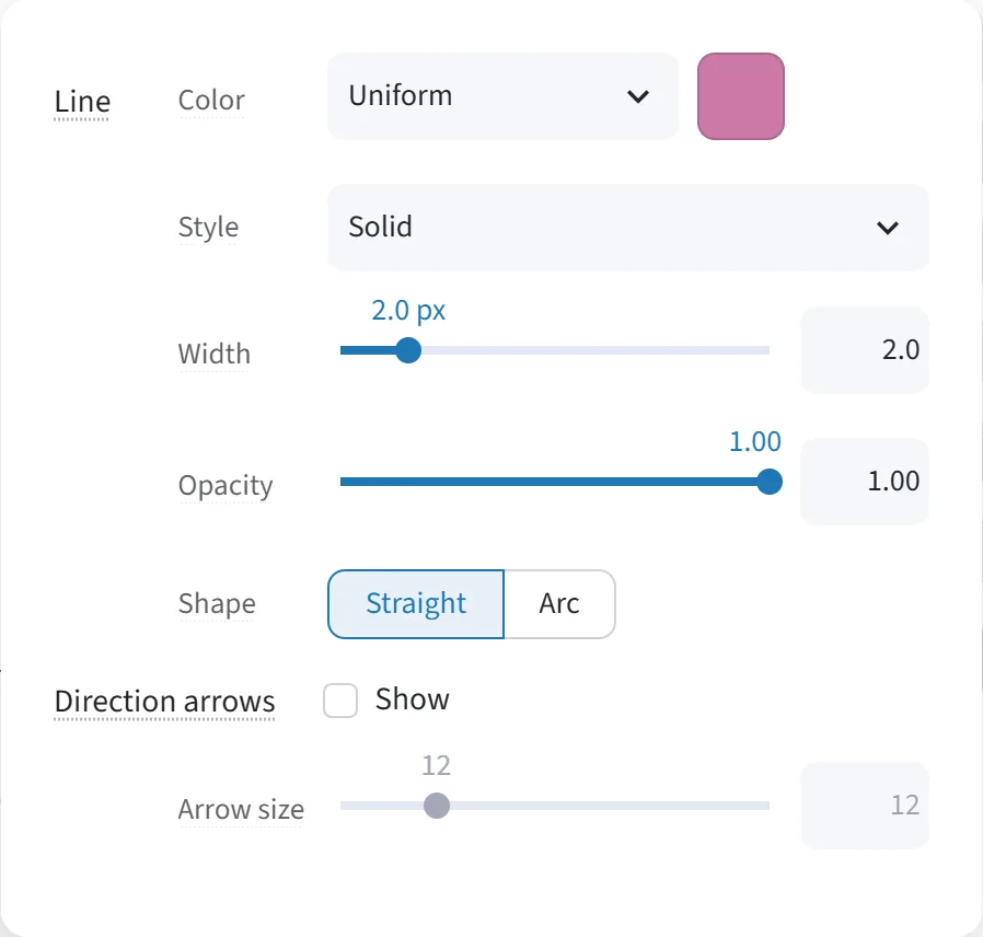
The Saccades switch draws the lines between fixations; its ▾ holds:

Control	What it does
Line → Color	Choose what decides the saccade color: one color for all; forward saccades and regressions in two colors; or a color per saccade type (forward, skip, refixation, return sweep, regression), with a legend. Forward / regression and by type need a word ID for each fixation, the word it landed on, mapped in your fixations table (such as EyeLink's CURRENT_FIX_INTEREST_AREA_ID); without one every saccade reads as other.
Line → color box	Choose the saccade line color.
Line → type colors	With By type: choose the color of each saccade type, such as regressions or return sweeps.
Line → Style	Choose the saccade line style: solid, dashed, dotted or dash-dot.
Line → Width	Set the saccade line width (thickness), in px.
Line → Opacity	Set the saccade line and arrow opacity; lower it to bring the fixations forward.
Shape	Choose the saccade shape: straight lines, or arcs over the text (a schematic, labelled Illustration).
Direction arrows → Show	Show saccade direction arrows: an arrowhead on each saccade, pointing where the eye went.
Direction arrows → Arrow size	Set the saccade arrowhead size.

Stimulus

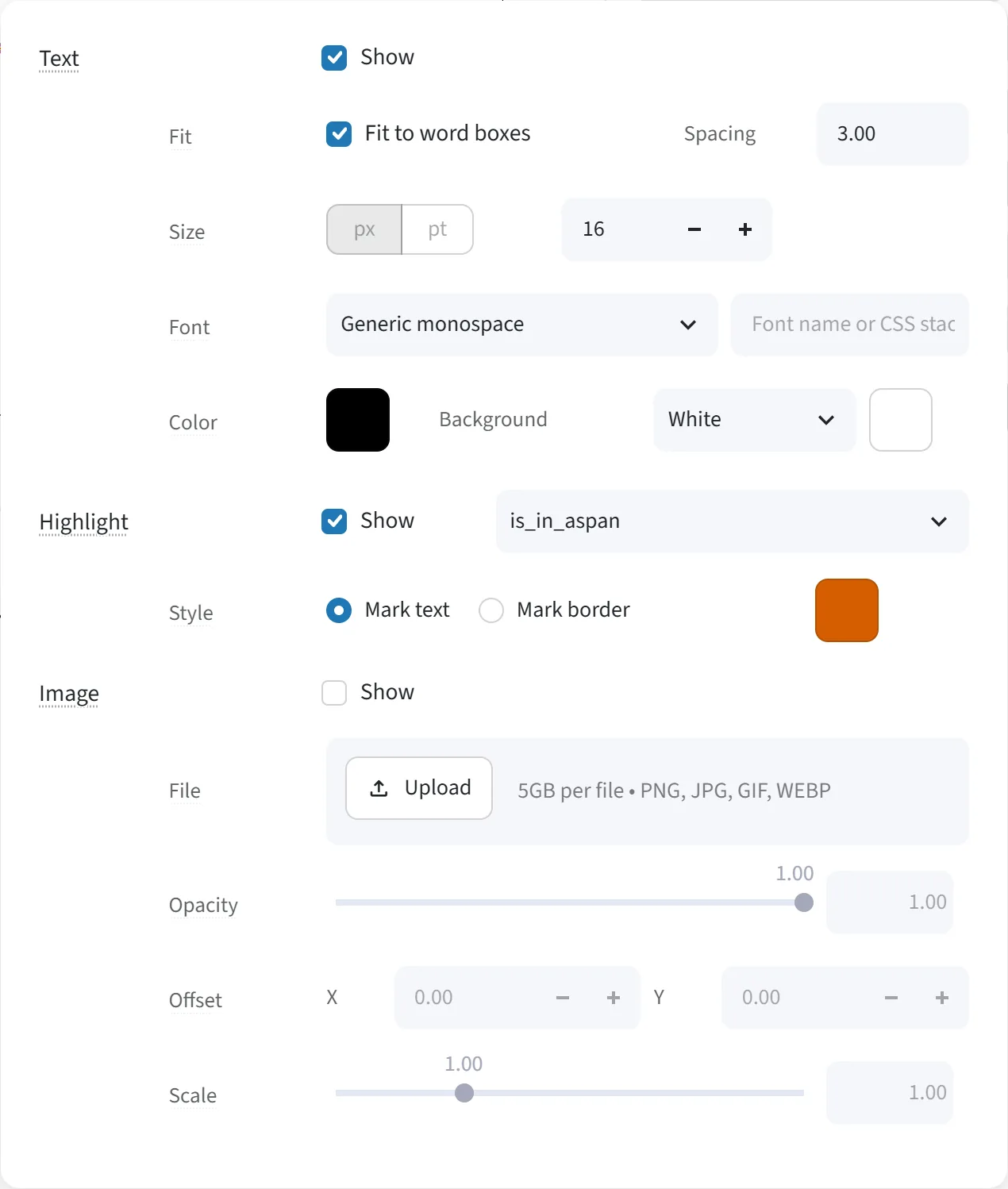
The Stimulus switch draws the text and the stimulus image; its ▾ holds:

Control	What it does
Text → Show	Show the stimulus text, the words the participant read, at their place on the screen.
Fit → Fit to word boxes	Size the stimulus text to fill its word boxes, instead of a fixed font size.
Spacing	Set the stimulus text line spacing: how far apart the lines are, in font sizes.
Size	Set the stimulus text font size, in px or pt.
Font	Choose the stimulus text font (typeface); Other… takes any font name.
Color → text color	Choose the stimulus text color.
Background	Choose the plot background color: a preset, or any color in the box beside it.
Highlight → Show	Highlight words in the stimulus text, such as the answer span.
Highlight → Highlight words by	Choose which words to highlight: a true/false word column, such as the critical span.
Style	Choose the word highlight style: colored text, or a border round the words; and the highlight color.
Image → Show	Show the stimulus image, the screen as shown in the experiment, under the scanpath.
File	Upload a stimulus image (PNG, JPEG, GIF or WebP) to draw under the scanpath.
Opacity	Set the stimulus image opacity; lower it so the scanpath reads over it.
Offset → X / Y	Move (nudge) the stimulus image left, right, up or down, in px, to line it up with the word boxes.
Scale	Resize (scale) the stimulus image so its text matches the word boxes.

Word boxes

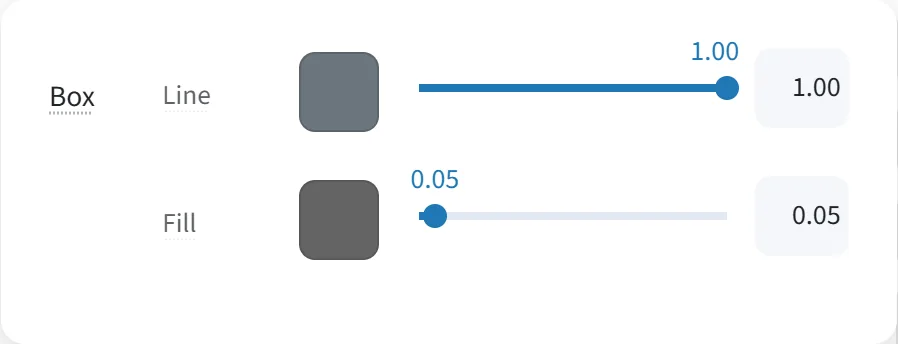
The Word boxes switch draws each word's interest area; its ▾ holds:

Control	What it does
Box → Line color	Choose the word box outline (border) color.
Box → Line opacity	Set the word box outline opacity; 0 hides the outlines.
Box → Fill color	Choose the word box fill color, inside each box.
Box → Fill opacity	Set the word box fill opacity; 0 draws outlines only.

Heatmap

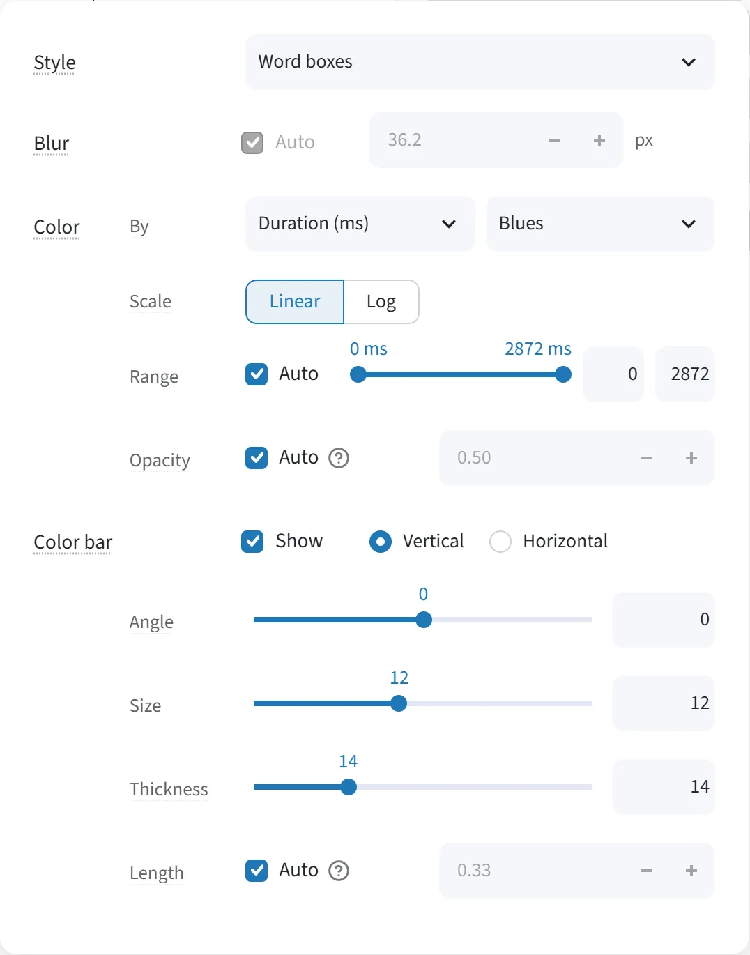
The Heatmap switch shows where reading concentrated; its ▾ holds:

Control	What it does
Style	Choose the heatmap style: colored word boxes, a smooth interpolated map, or fixation density.
Blur	Set the heatmap blur: how far each fixation spreads, for the smooth styles; Auto picks it.
Color → By	Choose what the heatmap measures: total fixation duration (dwell time), or the number of fixations.
Color → Colors	Choose the heatmap colors (color scale).
Scale	Choose a linear or log heatmap scale.
Range	For word-box heatmaps, fix the color range across trials. Auto fits each trial. Interpolated heatmaps use each figure's own peak.
Opacity	Set the heatmap opacity; Auto uses each style's own.
Color bar → Show, orientation, Angle, Size, Thickness, Length	Show the heatmap color bar, and set its orientation, label angle and size, thickness and length.

Raw gaze

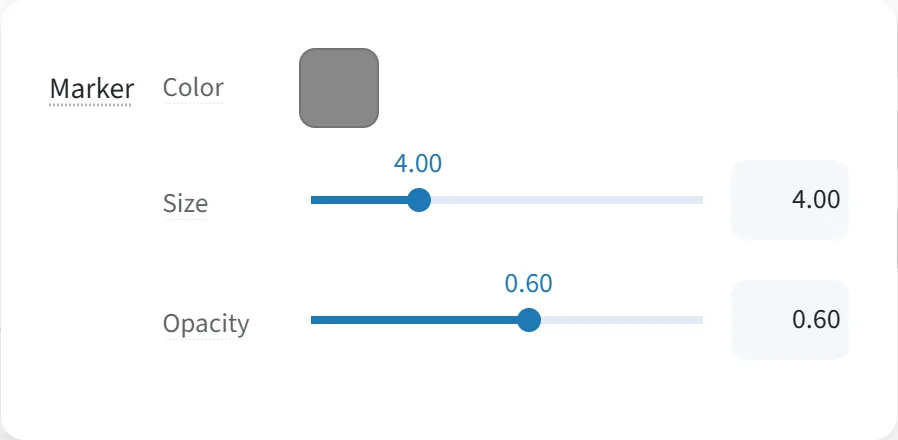
The Raw gaze switch draws the gaze samples as recorded; its ▾ holds:

Control	What it does
Marker → Color	Choose the raw gaze sample color.
Marker → Size	Set the raw gaze sample marker size.
Marker → Opacity	Set the raw gaze sample opacity.

Filters & highlights

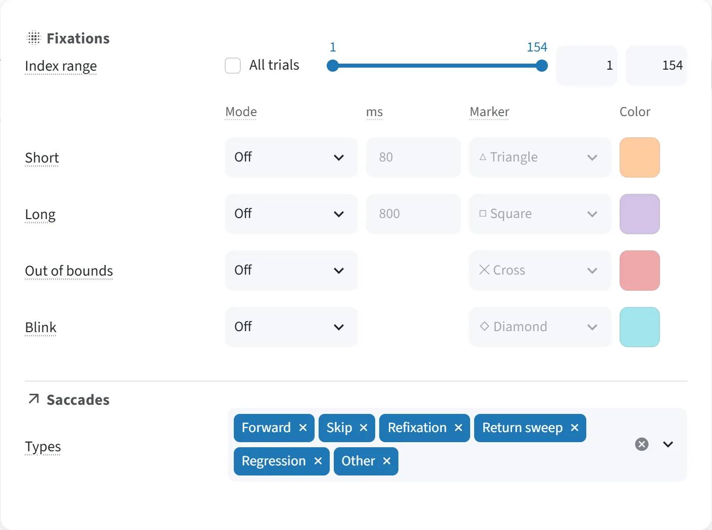
Which fixations and saccades are drawn, and which stand out:

Control	What it does
Fixations → Index range	Show only some fixations: a range of the reading order, such as fixations 10 to 40.
Fixations → All trials	Keep that fixation range when you move to another trial; otherwise it applies to this trial only, and the next trial shows all its fixations.
Short / Long	Find short or long fixations by a duration threshold (ms): Highlight marks them, Discard hides them.
Out of bounds	Highlight or discard out-of-bounds fixations, which land in no word box.
Blink	Highlight or discard fixations at or next to a blink (needs a blink column).
marker and color	Choose the marker shape and color of each highlighted fixation kind.
Saccades → Types	Show only some saccade types, such as regressions or return sweeps. Needs a word ID for each fixation, as for coloring saccades by type.

Figure & canvas

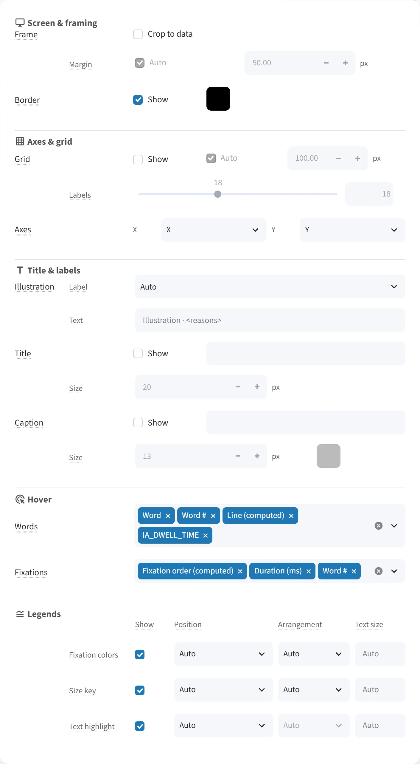
The figure as a whole:

Control	What it does
Frame → Crop to data	Crop (zoom) the figure to the part of the screen with data, instead of the whole screen.
Margin	Set the crop margin: the space round the data when cropping; Auto uses 5%.
Border → Show, color	Show the border line round the plot area, and choose its color. It marks the edge of the screen, or, with Crop to data, the edge of the cropped area.
Grid → Show	Show pixel grid lines (a coordinate grid) over the screen.
Grid → Auto, interval	Set the grid spacing (interval), in px, or let Auto choose it.
Labels	Set the grid label (tick label) font size.
Axes → X / Y	Choose the x and y axis fields. X / Y draws the reading on the screen. Any other pair turns the figure into a scatter plot (chart) of the fixations, with no text, word boxes or saccades, keeping the marker colors and sizes. For example: Time (ms) against X for a time course of the reading, where regressions show as dips; Time (ms) against Word # for reading progress through the text; Fixation # against Duration (ms) for fixation durations over the trial.
Illustration → Label	Choose when to label the figure as a manual illustration, not the recorded positions: when a setting changes its geometry (such as snapping fixations to a line or drawing saccades as arcs), always, or never.
Illustration → Text	Write the Illustration label's text.
Title → Show, text, Size	Add a figure title above the plot, and set its font size; {field} inserts a value of the trial.
Caption → Show, text, Size, color	Add a figure caption below the plot, and set its font size and color.
Hover → Words / Fixations	Choose the hover fields: what the tooltip shows when the mouse is over a word or a fixation.
Legends → Show	Show or hide each legend: Compare (A/B), Saccade types, Fixation colors, Size key or Text highlight.
Legends → Position	Choose the legend position: a corner, the middle of an edge, or down a side, outside or inside the plot.
Legends → Arrangement	Choose the legend arrangement: items stacked or side by side.
Legends → Text size	Set the legend text (font) size, in px.

Reset visualization

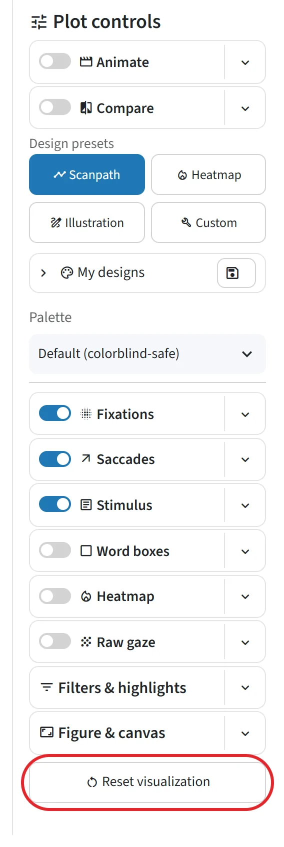
The button at the foot of the column.

Control	What it does
Reset visualization	Reset all plot settings to the defaults. Annotations, filters, data and the selected trial stay.

In Compare

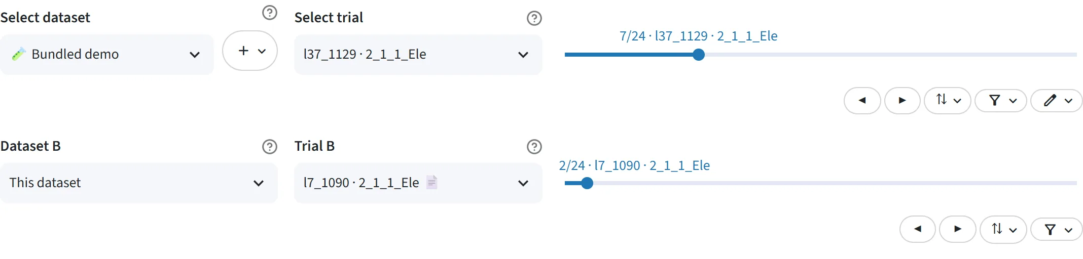
With Compare on, scanpath B gets a row of its own, and several menus split into a Scanpath A and a Scanpath B group.

Control	What it does
Dataset B	Choose the dataset scanpath B comes from: this one, or another dataset.
Trial B, slider, ◀ ▶	Choose scanpath B's trial: 📄 marks the same text, 👤 the same participant.
⇅ on B's row	Sort scanpath B's trial list, apart from A's. By default, trials of the same text as A come first, then the same participant, then the rest; or sort by any field, as on A's row.
on B's row	Filter scanpath B's trials, apart from A's.
Fixations ▾ → Scanpath A / B → Color, Size, Opacity	Choose each scanpath's fixation marker color, size range and opacity.
Saccades ▾ → Scanpath A / B → Color, Style, Width	Choose each scanpath's saccade line color, style and width.
Word boxes ▾ → Scanpath A / B → Line, Fill	Choose each scanpath's word box outline and fill colors and opacities.
Heatmap ▾ → Scanpath A / B → Colors	Choose each scanpath's heatmap colors (color scale).
Raw gaze ▾ → Scanpath A / B → Color	Choose each scanpath's raw gaze sample color.
Filters & highlights ▾ → · B groups	Set scanpath B's own fixation range, fixation highlights and saccade types.

Under the plot

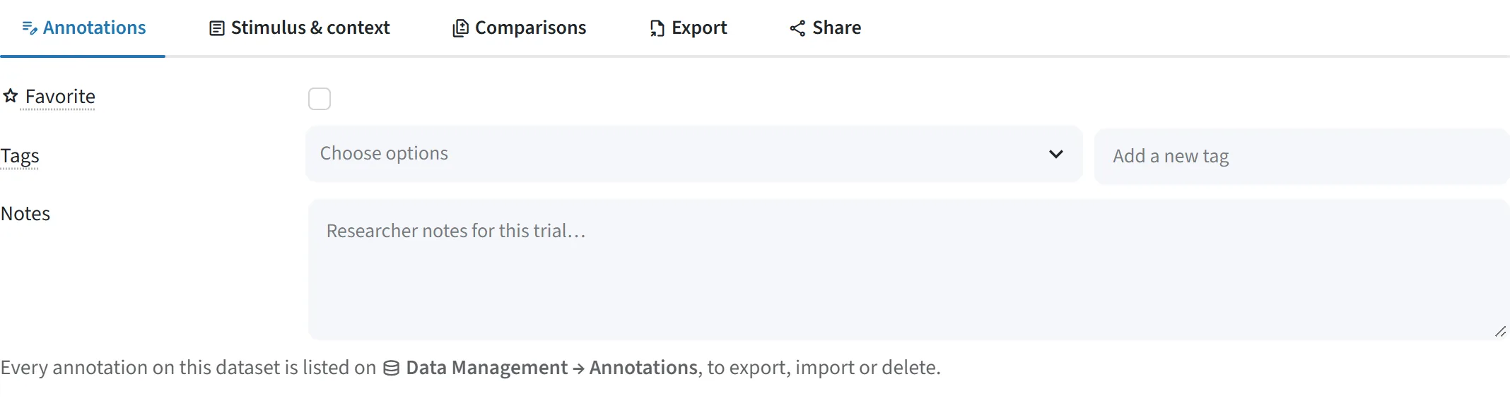
The tabs under the figure:

Tab	Control	What it does
Annotations	Favorite	Star the trial as a favorite, to find it again with the favorites filter.
	Tags / Add a tag	Tag the trial, with an existing tag or a new one, such as exclude. Tags let you filter the trial list later: the in the trial control bar keeps or hides trials by tag.
	Notes	Write a free-text note on the trial.
Stimulus & context	Context fields	Choose the trial context to show, such as the text's title, a question or an answer.
	Highlighted spans	Choose true/false word columns to highlight in the text, each with a summary.
Comparisons	Match field	Compare with other trials: show the trials that share this trial's value of a field, such as the same text.
	Columns	Set how many comparison panels per row.
Export	Download format	Export (download) the figure on screen as PNG, SVG, PDF or HTML, or the animation as an HTML, GIF or MP4 video.
	Width, unit, DPI	Set the PNG export size for print: width, unit and resolution (DPI).
	Trials to include	Choose which trials to export in the bundle: this one, the filtered trials, or all of them.
	Formats / Tabular data	Choose the bundle's figure formats and the data tables (CSV or Parquet) to include.
	Separable layers	Export each visual layer (fixations, saccades, word boxes…) as its own file, to stack in a vector editor.
	Annotations (JSON) / Settings file (JSON)	Settings file: beside each trial's figure, a plot_config.json recording how it was drawn (layers, colors, sizes, screen, title and caption), so the figures are documented. Annotations: one annotations.json with the exported trials' favorites, tags and notes, which Data Management → Annotations can import again.
	File path pattern	Set the file names inside the export bundle.
	Build export	Build the export bundle (a zip) to download.
Share	Link	Copy a share link that reopens this trial with these settings. The data doesn't travel in the link: whoever opens it needs the same dataset. The bundled demo works anywhere; a public corpus has to be downloaded on their side; for your own dataset, send its files and setup file ( Edit dataset → Download setup file) so they can add it first. A link made on your own computer (a localhost address) opens only where the app runs at that same address.
	Code → Flavour, Show every option	Get the Python or command-line code that redraws this figure, for scripts and reproduction.
	File → Download settings / Restore settings	Save the plot settings to a file, or load (restore) a saved settings file.